Independent research · Funds · ETFs · Public information only
Originally written August 2026 · Updated October 2026
Leveraged and inverse ETF decay
A daily-reset fund delivers L× the daily return, not L× the period return, so its median decays with volatility: a 2× fund on a 90%-vol stock loses 58% in a year the stock ends flat. Real prices add costs far above headline fees, and show the reset wins in calm trends and loses in chop.
Flat year, 2× at 90% vol
−58.0%
Stock ends flat · August result reverified
Single-stock 2× cost
7–34%/yr
Beyond T-bills · vs 2–4% for index funds
Sleeve vs 2× its stock
8 of 11
Corgi funds trailing since launch
TQQQ 2010–19
+4,373%
vs +1,276% for static 3×
Independent research written in a personal capacity. Not prepared for, reviewed by, or affiliated with any employer, client or institution. Not investment advice. Every data-derived figure was recomputed from public sources.
Summary
- Where this comes from. In August I wrote a simulation study of volatility drag in 2× daily-reset funds, built around the eleven single-stock funds in Corgi’s crypto and fintech sleeve. This note re-runs every number in it, corrects what was wrong, and tests the theory against real fund prices: twenty years of index funds (SSO, UPRO, SDS, SPXU, QLD, TQQQ, SQQQ, TNA, TZA), sector and Treasury funds (SOXL, SOXS, TMF, TMV), single-stock funds (TSLL, NVDL, CONL, MSTU), the Corgi sleeve itself since its June–July 2026 launch, and the VIX futures product UVXY.
- The mechanic is exact, not a rule of thumb. Over any window, a frictionless daily-reset fund’s log return equals L times the underlying’s log return minus ½(L² − L) times realised variance, plus a small skewness term. On 1-year windows of the S&P 500 since 1928, the fitted slope is −1.00 for 2× (theory −1) and −3.05 for 3× (theory −3), with R² of 0.996 and 0.988.
- The August results hold up. All eight closed-form flat-year losses reconcile to the tenth of a percent, and the simulated medians, break-evens and tail probabilities reproduce within Monte Carlo noise. At 90% volatility a 2× fund still loses about 58% in a year that ends flat, and the underlying must rise about 55% for the fund to break even.
- What I got wrong. (1) The 1.08% fee I used belongs to a different Corgi fund, FDRX. The crypto and fintech sleeve charges 0.20% or 0.45%. (2) The fee turns out to be the smallest cost. Real single-stock 2× funds lose a further 7–34% a year beyond fee and T-bill financing (TSLL 7.2%, NVDL 8.3%, CONL 12.1%, MSTU 34.2%), against 2–4% on index funds. (3) My gap-risk sigma count was computed on simple rather than log returns, so a one-day 50% fall at 90% volatility is a 12.2σ event under the lognormal model I stated, not 8.8σ. (4) The volatility band was a scenario. It is now measured: trailing 1-year volatility across the eleven underlyings runs from 56% to 113%, median 85%.
- The sleeve since launch. From first trade to 15 October 2026, eight of the eleven funds returned less than 2× their stock (one by a hair). The three exceptions are stocks that fell hard, where the daily reset cushions losses. Pooled, the funds trail a frictionless 2× reset by about 15% a year (naive s.e. ≈ 6pp) after only 66–77 trading days.
- Tracking error depends on the horizon. Against “L × index”, the median miss is 0.0pp at one day and −0.3 to −0.9pp at one month on long index funds. At one year it is −4 to −16pp, and long index funds trail L × index in 68–81% of rolling 1-year windows. At five years the dispersion is enormous: TQQQ’s 5th–95th percentile gap is −189pp to +573pp. Over five years, “L × index” stops being a benchmark and becomes a description of the path.
- The decay is not always a loss. In a low-volatility trend, daily reset beats static leverage by a wide margin: TQQQ returned +4,373% over 2010–19 against +1,276% for static 3×. It also beats static leverage in crashes, because the fund cannot go below zero. It loses in chop: in the flat, 20%-volatility stretch from May 2015 to June 2016, TQQQ lost 18% while the Nasdaq-100 lost 1%. For 3× at 20% volatility, static leverage wins whenever the 1-year index return lands between −13% and +35%, which covers most years.
- The leverage multiple matters, and the reset interval mostly does not. Weekly or monthly resets leave the drag almost unchanged in simulation. In history they add gap risk: a quarterly-rebalanced 3× S&P portfolio was wiped out in November 2008, and an annual one in October 1937. Going from 2× to 1.5× cuts drag by 62.5%, and at 90% volatility a 1.5× fund carries the drag of a 2× fund on a 55%-volatility stock.
- What follows for holders and alternatives. Breakeven volatility for a 3× fund to beat the unlevered index is about 15% at a 6% equity premium, close to the S&P 500’s long-run average, which is why broad 3× funds are a coin-flip bet on the volatility regime. For holdings beyond weeks, futures (financing near SOFR) and deep in-the-money LEAPS give leverage without daily reset. Margin is limited by Reg T and costs SOFR plus 1.5–2.5% at a low-cost retail broker. A volatility-targeted constant-leverage portfolio cut the worst drawdown of 3× S&P from −99% to −75% in the 1934–2026 backtest.
What this note does, and what changed since August
The August study made one argument. Daily-reset leverage was designed for indices with 15–30% volatility. Applied unchanged to single stocks running at 70–120%, it produces a product that can be right about direction and still lose money. I modelled that with geometric Brownian motion (GBM), zero drift, and a scenario band of volatilities, because at the time the funds had traded for only a few weeks.
Two months on, more of this can be measured. The eleven Corgi crypto and fintech funds have 66–77 trading days of prices. Their underlyings have years of daily data. Older 2× single-stock funds on the same kind of names (CONL on Coinbase since 2022, MSTU on Strategy since 2024) and twenty years of index-based leveraged and inverse ETFs give a much larger sample of how the wrapper behaves against “L × index”. This note therefore does four things:
- Verifies every figure in the August Part I by re-running it from scratch (Section 3, Appendix A).
- Corrects the errors: the wrong fee, the missing swap spread, the sigma arithmetic and a loose equivalence claim (Section 3).
- Measures what was assumed: realised volatility, all-in costs, tracking at 1 day, 1 month, 1 year and 5 years, and outcomes across regimes (Sections 4–6).
- Extends the analysis: when daily reset beats static leverage, breakeven volatility, rebalancing frequency, gap risk under fat tails, volatility products, and the alternatives (Sections 7–13).
The mechanic
2.1 Two days, four numbers
A leveraged fund targets a multiple of the underlying’s daily return, not of its return over the holding period. Holding leverage constant forces the fund to rebalance every session. After the underlying rises, exposure has drifted below target and the fund buys; after it falls, the fund sells. Two days are enough to show the cost:
| Underlying | 2× daily fund | |
|---|---|---|
| Start | 100.00 | 100.00 |
| Day 1, +10.00% | 110.00 | 120.00 |
| Day 2, −9.09% | 100.00 | 98.18 |
| Net | 0.00% | −1.82% |
The fund met its objective on both days, the underlying finished flat, and the fund lost 1.8%. Nothing malfunctioned; this is how the wrapper works. The same arithmetic punishes an inverse fund: a −1× fund on the same two days goes 100 → 90 → 98.18.
2.2 Continuous time, with financing
Let the underlying follow dS/S = μ dt + σ dW, and let the fund deliver L times the daily return, pay financing r on the borrowed (L − 1) and carry other costs c (fee plus swap spread). Applying Itô’s lemma to both:
d ln F   = [ r + L(μ − r) − c − ½ L² σ² ] dt + L σ dW
L d ln S = [ L μ − ½ L σ² ] dt               + L σ dW

drag  =  d ln F − L d ln S  =  [ −(L − 1) r − c − ½ (L² − L) σ² ] dt
The volatility term ½(L² − L)σ² is the decay. It is −σ² a year for L = 2, −3σ² for L = 3, −σ² for L = −1 and −6σ² for L = −3. It is zero only at L = 0 and L = 1. Inverse funds decay faster than long funds of the same absolute multiple, because L² − L is larger when L is negative.
A common way to state this uses two approximations: the fund grows at about Lμ − L²σ²/2 (before financing), whereas a naive reader expects L(μ − σ²/2), L times the index’s compound growth. The difference is exactly the ½(L² − L)σ² term above. Two things follow from it:
- Drag scales with variance, not volatility. Tripling volatility multiplies the drag by nine. A rule of thumb calibrated on a 15% index is useless on a 90% stock.
- The expected value is not decayed; the median is. Under GBM, E[F(T)] = exp{[r + L(μ − r) − c]T}. The mean grows at the full levered drift. What collapses is the typical path: the terminal distribution is lognormal with log-variance L²σ²T, so the mean is carried by a few very strong paths. A shareholder holds one path, not the average.
2.3 The exact discrete relation, and path dependence
The continuous-time result is an approximation to an identity that holds exactly over any window of n days. With daily underlying returns ri and no frictions,
ln(F_T/F_0) − L·ln(S_T/S_0) = Σ [ ln(1 + L·r_i) − L·ln(1 + r_i) ]
                            = −½(L² − L)·Σ r_i²
                              + ⅓(L³ − L)·Σ r_i³
                              − ¼(L⁴ − L)·Σ r_i⁴ + …
The first term is realised variance. The second is a skewness term: for L = 2 it is +2Σr³, so a market with large down days (negative Σr³) loses slightly more than variance alone predicts. Two consequences:
- The fund’s terminal value depends on the path only through realised moments. Two paths with the same endpoint and the same realised variance give, to second order, the same fund value. This is path dependence in a precise sense: the endpoint does not determine the outcome, but the endpoint plus realised variance nearly does.
- It can be checked on real data. Figure 1 plots the frictionless log gap against realised variance for every 1-year window of the S&P 500 since 1928. The fitted slopes are −1.00 (L = 2; theory −1), −3.05 (L = 3; theory −3), −1.00 (L = −1) and −6.19 (L = −3; theory −6). The quadratic term alone explains 99.6% of the variation for 2× and 98.8% for 3×; adding the cubic term raises this to 99.9% and 99.6%. For −3× the slope is steeper than the quadratic theory because the higher-order terms grow quickly with |L|, and the fourth-order term, −¼(L⁴ − L)Σr⁴, rises with fat-tailed days.
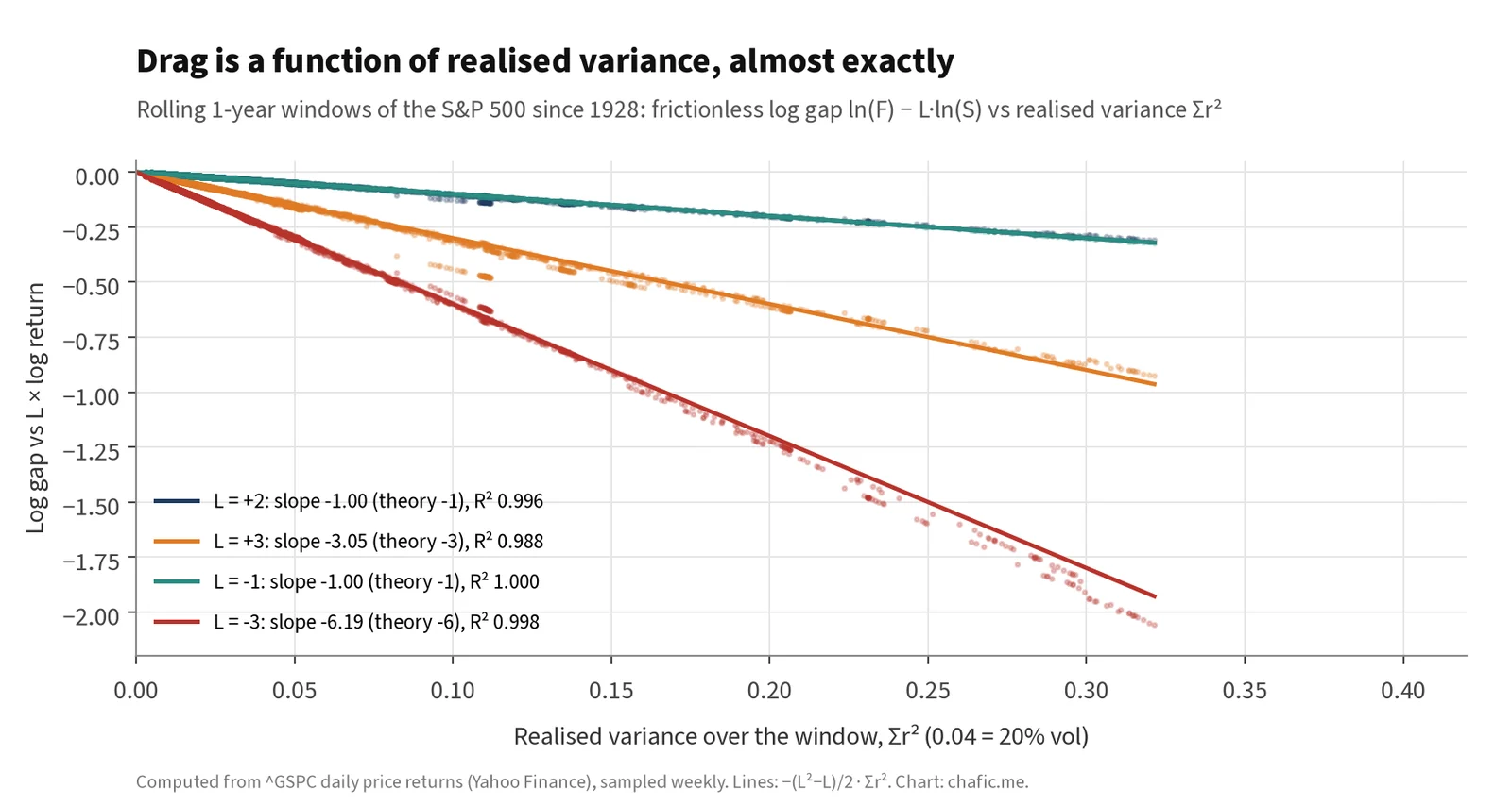
Figure 1. Drag tracks realised variance almost exactly. Rolling 1-year windows of the S&P 500 price index, 1928–2026. Computed from Yahoo Finance daily data.
Verifying the August results
The August simulation used 60,000 GBM paths per volatility level, 252 steps a year, zero drift, NAV floored at zero, a 1.08% fee and 4.75% financing on the borrowed notional. I rebuilt it independently and ran it with the original inputs. The headline numbers reproduce:
| Vol | Flat year: note | Flat year: recomputed | Median: note | Median: recomputed | P(fund<0 given und>0): note | recomputed | Break-even: note | recomputed |
|---|---|---|---|---|---|---|---|---|
| 15% | −7.8% | −7.8% | −9.7% | −10.0% | 21.8% | 22.2% | 4.1% | 4.1% |
| 30% | −13.8% | −13.8% | −21.2% | −21.4% | 21.7% | 21.2% | 7.7% | 7.7% |
| 45% | −23.0% | −23.0% | −37.4% | −37.4% | 26.5% | 25.8% | 13.9% | 13.9% |
| 60% | −34.2% | −34.2% | −54.1% | −54.5% | 32.6% | 32.3% | 23.3% | 23.3% |
| 75% | −46.2% | −46.2% | −69.3% | −69.7% | 39.2% | 39.0% | 36.4% | 36.4% |
| 90% | −58.0% | −58.0% | −81.7% | −81.7% | 45.5% | 46.7% | 54.4% | 54.4% |
| 105% | −68.7% | −68.7% | −89.8% | −89.9% | 52.9% | 54.1% | 78.7% | 78.7% |
| 120% | −77.6% | −77.6% | −94.9% | −95.0% | 60.0% | 60.6% | 111.5% | 111.5% |
Table 1. August note (as printed) vs independent re-run with the note’s own inputs. Closed form exp(−σ²T − cT) − 1 for the flat year; break-even = exp[(σ² + c)/2] − 1. Probabilities differ by Monte Carlo noise of 1–2pp, as the note said they would.
The closed-form flat-year figures and break-evens match to the tenth of a percent, and the medians and probabilities sit within simulation noise. The two-year figure at 90% volatility (−83%) and the other horizons of Table A2 also reproduce, within about half a point. The mean-versus-median point stands. Under the note’s costs the population mean is exactly exp(−5.83%) − 1 = −5.7% at every volatility, and the sample means printed in the note (−5.2% to −7.3%, with the 105% cell at 0.0%) are, as it said, noise around that value.
Six things needed fixing:
- Wrong fee. The 1.08% is the fee of FDRX (Founder-Led 2x Daily ETF), a different fund in the same trust. The crypto and fintech funds list 0.20% (MSTC, COIX, HOOC) or 0.45% (the other eight) [1][2].
- Incomplete financing model. A swap-based 2× fund pays the swap dealer a rate plus a spread on the full notional and earns collateral income on its own equity. Net, it pays roughly the short rate on (L − 1) plus the spread on L. The refresh uses SOFR (3.88% on 14 October 2026) on the borrowed notional plus a 1.0% spread on the full notional as the base case. Section 5 shows the real spread on single stocks has been much larger.
- Gap-risk arithmetic. At 90% volatility the daily standard deviation is 5.67%, and 0.50/0.0567 = 8.8. Under the lognormal model the note specified, a one-day 50% fall is a log move of ln 0.5 = −0.693, which is 12.2 standard deviations. The conclusion survives, because the real distribution has jumps (Section 11), but the number was wrong.
- A loose equivalence. “At 90% volatility a 1.5× fund behaves about as forgiving as a 2× fund on 60%.” The drag of 1.5× at 90% is 0.375 × 0.81 = 0.30, which equals the 2× drag at 55% volatility, not 60%. Moving from 2× to 1.5× cuts drag by 62.5% (from 1.0σ² to 0.375σ²) while keeping 75% of the gross exposure and half of the extra exposure.
- “All tail figures are conservative.” This is only partly true. Bootstrapping each stock’s actual returns (Section 8) leaves the median and flat-year results almost unchanged and slightly lowers some negative-year probabilities. What it raises sharply is the chance of NAV being wiped out, from roughly zero under GBM to 5–19% for UPST, CIFR and IREN.
- Unverifiable claims removed. I dropped the statement that no competitor publishes a live drag figure and the shelf-size counts, because I could not verify them from public sources for this update.
With refreshed costs (0.45% fee, SOFR, 1.0% spread) the headline numbers barely move at high volatility: the flat year at 90% goes from −58.0% to −58.2%. Variance dominates cost above roughly 45% volatility, as the August note said. Appendix A has the full refreshed tables.
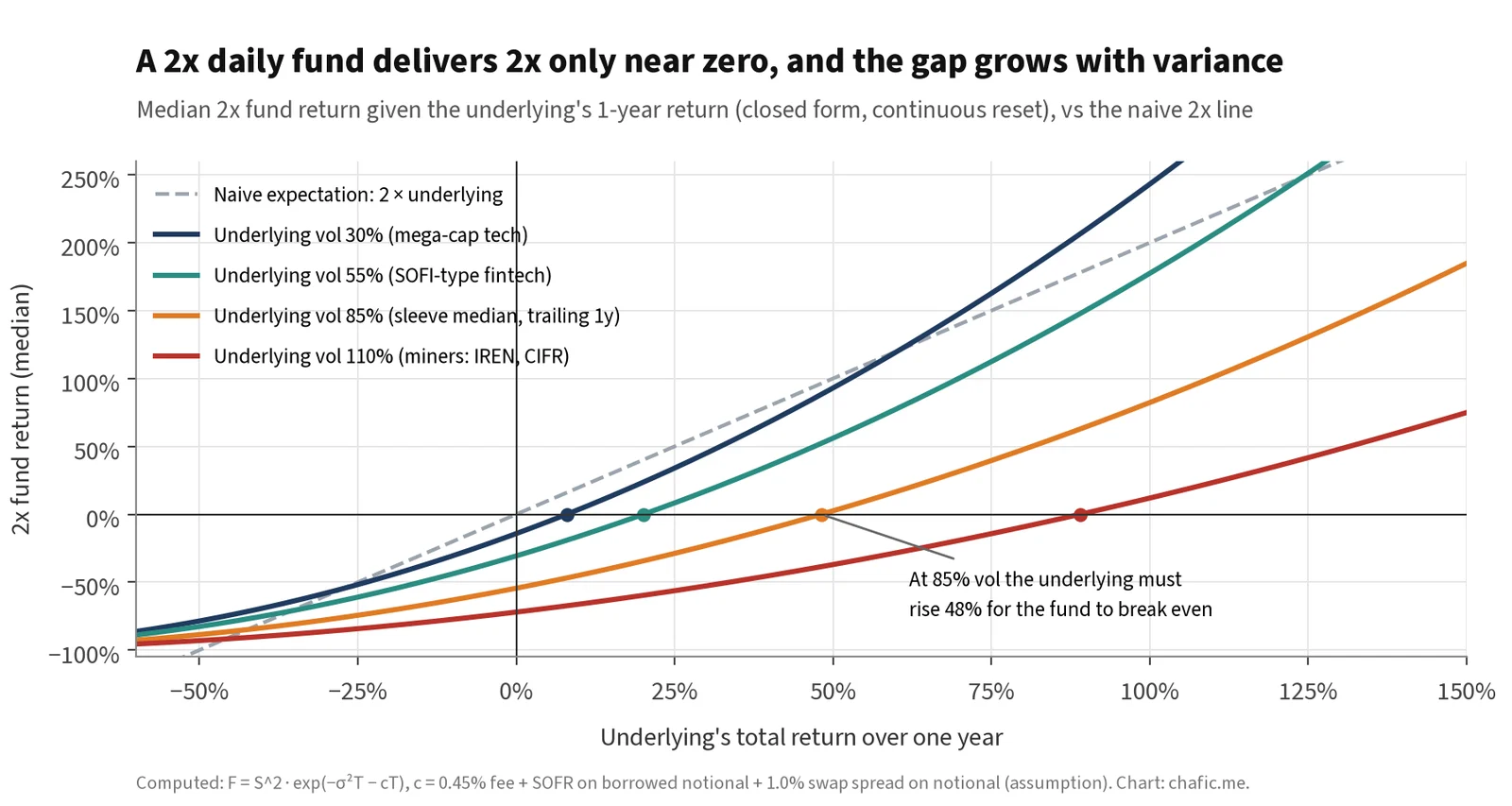
Figure 2. The payoff a 2× buyer expects is a straight line; the payoff delivered is a curve that bends further below it as variance rises. Closed form under GBM with refreshed costs.
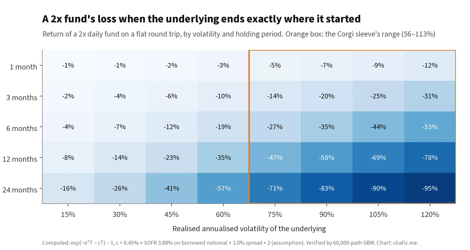
Figure 3. Refreshed version of the August Exhibit 1: 2× fund return on a flat round trip by horizon and volatility.
The case study, measured: Corgi's 2× crypto and fintech sleeve
4.1 Volatility is no longer a scenario
The August note had to treat volatility as an input. It can now be measured. Over the twelve months to 15 October 2026, the eleven stocks behind the sleeve had realised volatility between 56% (SOFI) and 113% (CIFR), with a median of 85% (Figure 4). The August scenario band of 70–120% was about right for the crypto names (MSTR, COIN, CRCL, MARA, BMNR, GLXY, IREN, CIFR: 72–113%). It was slightly high for the fintech names (HOOD 72%, UPST 65%, SOFI 56%). At the sleeve’s median volatility, a frictionless 2× fund gives up about 51% in a year that ends flat; at CIFR’s, about 72%.
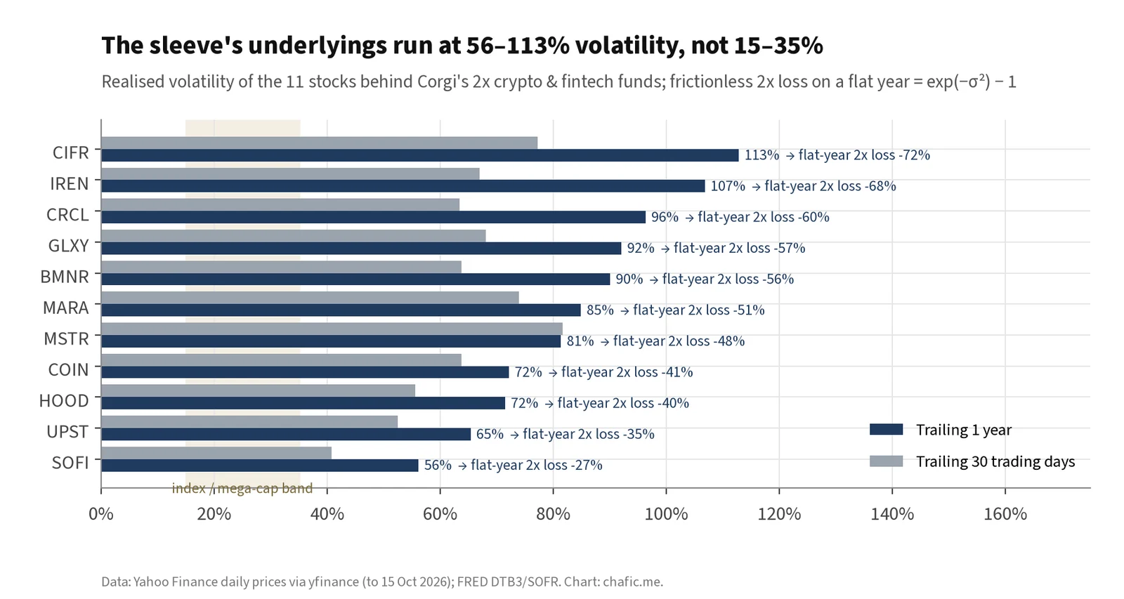
Figure 4. Realised volatility of the sleeve’s underlyings. Data: Yahoo Finance daily closes to 15 October 2026.
4.2 Performance since launch
The funds began trading between 26 June and 14 July 2026. Table 2 compares each fund’s market-price return to 15 October with its stock, with 2× the stock, and with a frictionless daily-reset 2× built from the stock’s own daily returns.
| Fund / underlying | First trade | Fee | Vol, 1y | Vol since launch | Underlying | 2 × underlying | Frictionless 2x | Fund | Residual cost, ann. (± s.e.) |
|---|---|---|---|---|---|---|---|---|---|
| MSTC / MSTR | 26 Jun | 0.20% | 81% | 84% | +83.8% | +167.6% | +178.6% | +162.5% | 20% (± 14%) |
| COIX / COIN | 26 Jun | 0.20% | 72% | 74% | +23.3% | +46.6% | +29.8% | +25.4% | 10% (± 16%) |
| CIR / CRCL | 7 Jul | 0.45% | 96% | 83% | +33.5% | +67.0% | +48.4% | +43.0% | 12% (± 21%) |
| MHX / MARA | 14 Jul | 0.45% | 85% | 91% | −31.5% | −63.0% | −61.8% | −63.0% | 14% (± 26%) |
| BNMC / BMNR | 10 Jul | 0.45% | 90% | 80% | +55.9% | +111.9% | +107.2% | +97.9% | 14% (± 23%) |
| GLX / GLXY | 30 Jun | 0.45% | 92% | 87% | −33.2% | −66.5% | −64.6% | −65.6% | 11% (± 17%) |
| IREC / IREN | 14 Jul | 0.45% | 107% | 108% | −21.2% | −42.5% | −52.7% | −56.5% | 37% (± 26%) |
| CIFC / CIFR | 30 Jun | 0.45% | 113% | 123% | −59.0% | −118.0% | −89.4% | −89.8% | 19% (± 25%) |
| HOOC / HOOD | 10 Jul | 0.20% | 72% | 70% | −7.1% | −14.3% | −23.5% | −26.1% | 10% (± 9%) |
| SOFC / SOFI | 10 Jul | 0.45% | 56% | 52% | −19.6% | −39.3% | −40.0% | −41.9% | 11% (± 12%) |
| UPSC / UPST | 10 Jul | 0.45% | 65% | 50% | −24.4% | −48.8% | −46.6% | −48.0% | 8% (± 15%) |
Table 2. Corgi 2× crypto and fintech funds from first trade to 15 October 2026. “Residual cost” is the annualised mean of fund return − [2 × stock return − 1 × T-bill], so it includes the fee, the swap spread and any price-vs-NAV noise. Fees: issuer site and Yahoo Finance [1][2].
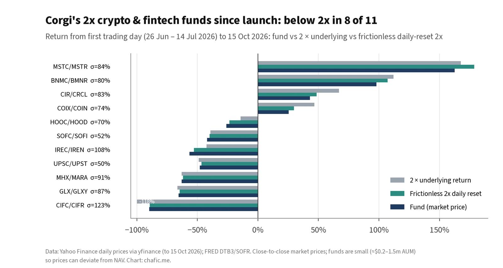
Figure 5. Fund vs 2× underlying vs frictionless 2× daily reset since launch.
Three readings:
- Compounding cuts both ways, even over three months. MSTR rose 84% on a strong trend, and frictionless daily reset would have beaten 2× (+179% against +168%). CIFR fell 59%, and 2× its return would be −118%, which is impossible. Reset held the fund to −90%. Stocks that chopped (COIN +23%, CRCL +34%) are where the gap to 2× is largest: COIX returned +25% against a naive +47%.
- Eight of eleven funds returned less than 2× their stock (MHX by under a tenth of a point). The three that did better are GLX, CIFC and UPSC, all on stocks that fell 24–59%, where the daily reset cushions the loss.
- Costs beyond the fee are large but not yet measurable fund by fund. Pooled across the eleven funds, the residual cost runs at about 15% a year. That is noisy: with only ~70 days of 50–120%-volatility returns, each fund’s standard error is 9–26pp, and the naive pooled standard error is about 6%pp. Some of it is closing-price noise in funds with $0.2–1.5m of assets. The older funds in Section 5 show the same pattern with much tighter errors.
Twenty years of real funds: tracking and costs
5.1 What the funds actually charge
For every fund I compute the daily residual: fund return minus L × underlying return plus (L − 1) × T-bill. If the fund delivered exactly L times the underlying’s daily total return and financed at T-bills, the residual would average zero. Its annualised mean is the all-in cost beyond T-bill financing: fee, swap spread, transaction costs and any timing mismatch. Dividing the excess over the fee by |L| gives an implied spread per unit of notional.
| Fund | Target | Underlying | Since | Net fee | Und. vol | Residual cost ± s.e. | Implied spread | Fund CAGR | Und. CAGR | $1 became | $1 at L × und. |
|---|---|---|---|---|---|---|---|---|---|---|---|
| SSO | +2x | S&P 500 TR | 2006 | 0.84% | 19% | 2.0% ± 0.8% | 0.6% | 15.8% | 11.5% | $19 | $17 |
| UPRO | +3x | S&P 500 TR | 2009 | 0.88% | 17% | 2.5% ± 0.8% | 0.5% | 32.8% | 15.2% | $134 | $33 |
| SH | −1x | S&P 500 TR | 2006 | 0.88% | 19% | 0.6% ± 0.4% | −0.2% | −11.2% | 11.5% | $0.09 | below $0 |
| SDS | −2x | S&P 500 TR | 2006 | 0.91% | 19% | 0.8% ± 0.8% | 0.0% | −25.0% | 11.6% | $0.00 | below $0 |
| SPXU | −3x | S&P 500 TR | 2009 | 0.90% | 17% | 1.0% ± 0.9% | 0.0% | −42.3% | 15.2% | $0.00 | below $0 |
| QLD | +2x | Nasdaq-100 | 2006 | 0.89% | 22% | 2.0% ± 0.9% | 0.5% | 25.1% | 16.7% | $94 | $45 |
| TQQQ | +3x | Nasdaq-100 | 2010 | 0.78% | 21% | 3.0% ± 0.7% | 0.7% | 42.4% | 19.7% | $360 | $57 |
| PSQ | −1x | Nasdaq-100 | 2006 | 0.95% | 22% | 1.0% ± 0.6% | 0.1% | −16.5% | 16.7% | $0.03 | below $0 |
| SQQQ | −3x | Nasdaq-100 | 2010 | 0.94% | 21% | 1.7% ± 0.8% | 0.3% | −52.7% | 19.7% | $0.00 | below $0 |
| TNA | +3x | Russell 2000 | 2008 | 1.05% | 24% | 3.6% ± 0.8% | 0.8% | 14.5% | 12.9% | $11 | $24 |
| TZA | −3x | Russell 2000 | 2008 | 0.99% | 24% | 4.1% ± 0.9% | 1.0% | −49.4% | 12.9% | $0.00 | below $0 |
| SOXL | +3x | Semis (SOXX) | 2010 | 0.75% | 31% | 4.3% ± 1.7% | 1.2% | 36.8% | 25.0% | $179 | $118 |
| SOXS | −3x | Semis (SOXX) | 2010 | 1.00% | 31% | 3.5% ± 1.4% | 0.8% | −70.7% | 25.0% | $0.00 | below $0 |
| TMF | +3x | 20y+ UST (TLT) | 2009 | 0.90% | 15% | 2.7% ± 0.9% | 0.6% | −6.9% | 1.7% | $0.29 | $2.04 |
| TMV | −3x | 20y+ UST (TLT) | 2009 | 0.97% | 15% | 1.9% ± 0.7% | 0.3% | −13.6% | 1.7% | $0.08 | below $0 |
| TSLL | +2x* | TSLA | 2022 | 0.83% | 58% | 7.2% ± 1.0% | 3.2% | −17.1% | 6.1% | $0.46 | n/m |
| NVDL | +2x* | NVDA | 2022 | 1.05% | 48% | 8.3% ± 2.7% | 3.6% | 133.0% | 92.0% | $25 | n/m |
| CONL | +2x* | COIN | 2022 | 1.04% | 83% | 12.1% ± 1.8% | 5.5% | −29.4% | 17.4% | $0.24 | n/m |
| MSTU | +2x | MSTR | 2024 | 1.05% | 86% | 34.2% ± 6.0% | 16.6% | −60.2% | 6.6% | $0.15 | $1.28 |
| UVXY | +1.5x* | VIX futures (VIXY) | 2011 | 1.23% | 69% | 6.5% ± 2.7% | 3.5% | −80.0% | −51.3% | $0.00 | n/m |
Table 3. Leveraged and inverse ETFs vs their benchmarks, from inception to 15 October 2026. Underlying total-return proxies: ^SP500TR for the S&P 500; QQQ, IWM, SOXX, TLT and VIXY adjusted closes plus their own fees for the others. Net fees from Yahoo Finance fund profiles retrieved 15 October 2026 (prospectus figures may differ slightly). *Leverage changed during the sample: TSLL 1.5× → 2× on 2 April 2024; NVDL and CONL 1.5× → 2× on 22 January 2024; UVXY 2× → 1.5× on 28 February 2018 [3][4][5]. The residual model uses the leverage in force each day.
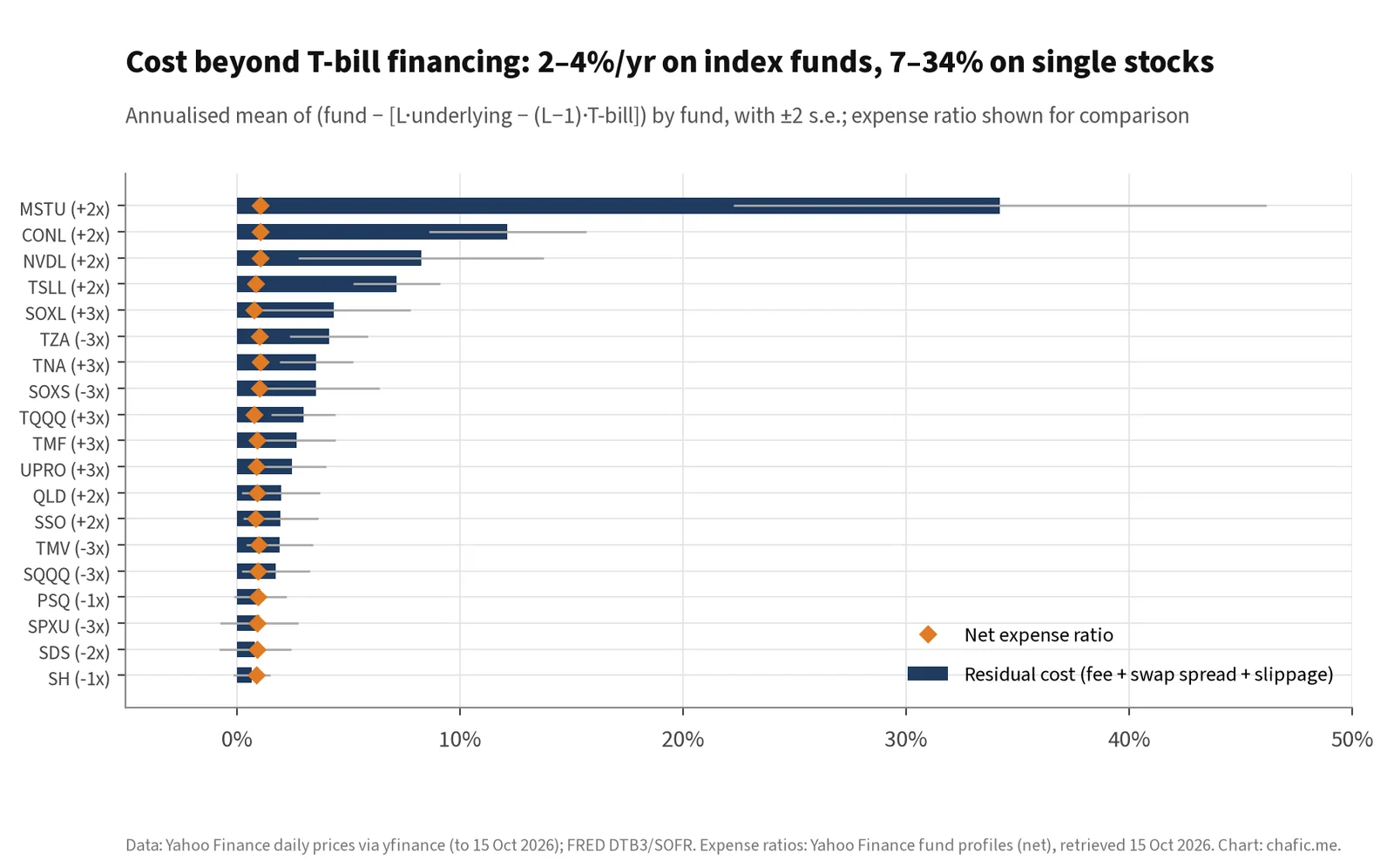
Figure 6. Residual cost beyond T-bill financing vs net expense ratio.
The pattern is clear:
- Index funds cost about fee plus 0.5–1% of notional. SSO, UPRO, QLD and TQQQ run at 2.0–3.0% a year beyond T-bills, an implied swap spread of 0.5–0.7% per unit of notional over the T-bill rate. Part of that is the gap between T-bills and the swap benchmark (SOFR or OBFR), not dealer margin. Small-cap and semiconductor funds cost more (TNA 3.6%, SOXL 4.3%).
- Inverse funds look cheap on this measure. SH, SDS and SPXU come in at or below their fees. A short swap receives the financing rate, and here the benchmark rate has sat slightly above T-bills; the spread works in the short holder’s favour. Their problem is drift and decay, not cost.
- Single-stock funds are expensive, and the fee hides it. TSLL costs 7.2% a year beyond T-bills on a 0.83% fee, NVDL 8.3% on 1.05%, CONL 12.1% on 1.04% and MSTU 34.2% on 1.05%. That implies swap spreads of 3–17% a year per unit of notional, which reflects how hard it is to borrow and hedge these names. The real cost of a 2× single-stock fund is the swap, and a 0.20–0.45% headline fee says little about it.
Table 4 shows how sensitive the August flat-year numbers are to the spread. At 90% volatility, moving from no spread to a CONL-like 5.5% changes the flat-year loss from −57% to −62%. At 30% volatility, the same change takes it from −12% to −22%. Costs matter most where the drag matters least.
| Swap spread on notional | All-in carry, 2x | Flat year at 30% vol | at 60% | at 90% | Break-even at 90% |
|---|---|---|---|---|---|
| 0.0% | 4.3% | −12% | −33% | −57% | 53% |
| 1.0% | 6.3% | −14% | −35% | −58% | 55% |
| 3.0% | 10.3% | −18% | −37% | −60% | 58% |
| 5.5% | 15.3% | −22% | −40% | −62% | 62% |
| 10.0% | 24.3% | −28% | −45% | −65% | 69% |
Table 4. 2× fund, 12-month flat round trip, by swap spread on notional (0.45% fee, SOFR on the borrowed half). Computed.
5.2 Tracking “L × index” at 1 day, 1 month, 1 year and 5 years
Table 5 reports the gap between each fund’s return and L times its underlying’s return over every rolling window: the median and, in brackets, the 5th and 95th percentiles, in percentage points.
| Fund | 1 day | 1 month | 1 year | 5 years | Share of 1y windows below L × index |
|---|---|---|---|---|---|
| SSO | 0.0 [0, 0] | −0.3 [−1, 0] | −3.9 [−14, +6] | −12.0 [−49, +56] | 81% |
| UPRO | 0.0 [0, 0] | −0.5 [−2, +1] | −8.3 [−36, +15] | −9.7 [−130, +188] | 75% |
| QLD | 0.0 [0, 0] | −0.3 [−1, 0] | −4.2 [−13, +7] | +12.4 [−66, +188] | 73% |
| TQQQ | 0.0 [0, 0] | −0.6 [−3, +1] | −9.0 [−35, +21] | +58.5 [−189, +573] | 68% |
| TNA | 0.0 [0, 0] | −0.7 [−3, +2] | −10.9 [−37, +28] | −95.4 [−176, +72] | 81% |
| SOXL | 0.0 [−1, 0] | −0.9 [−5, +4] | −16.4 [−79, +65] | −89.2 [−498, +1159] | 71% |
| TMF | 0.0 [0, 0] | −0.5 [−2, +1] | −6.6 [−18, +9] | −36.4 [−52, +19] | 81% |
| SPXU | 0.0 [0, 0] | +0.1 [−2, +3] | +6.8 [−25, +43] | +188.1 [+87, +278] | 37% |
| SQQQ | 0.0 [0, 0] | 0.0 [−4, +4] | +14.0 [−33, +61] | +295.9 [+180, +592] | 34% |
| TZA | 0.0 [0, 0] | −0.3 [−5, +5] | −3.4 [−52, +63] | +80.6 [−31, +317] | 54% |
| TSLL | 0.0 [0, 0] | −1.2 [−6, +7] | −24.0 [−86, +2] | – | 95% |
| NVDL | 0.0 [0, 0] | −1.3 [−5, +4] | −26.6 [−58, +187] | – | 59% |
| CONL | −0.1 [0, 0] | −2.3 [−7, +9] | −39.6 [−129, +139] | – | 76% |
Table 5. Fund return minus L × underlying return over rolling windows (percentage points; median [5th, 95th percentile]). Windows overlap daily. Inverse-fund 5-year numbers are mechanically positive because L × a large positive index return is far below −100%.
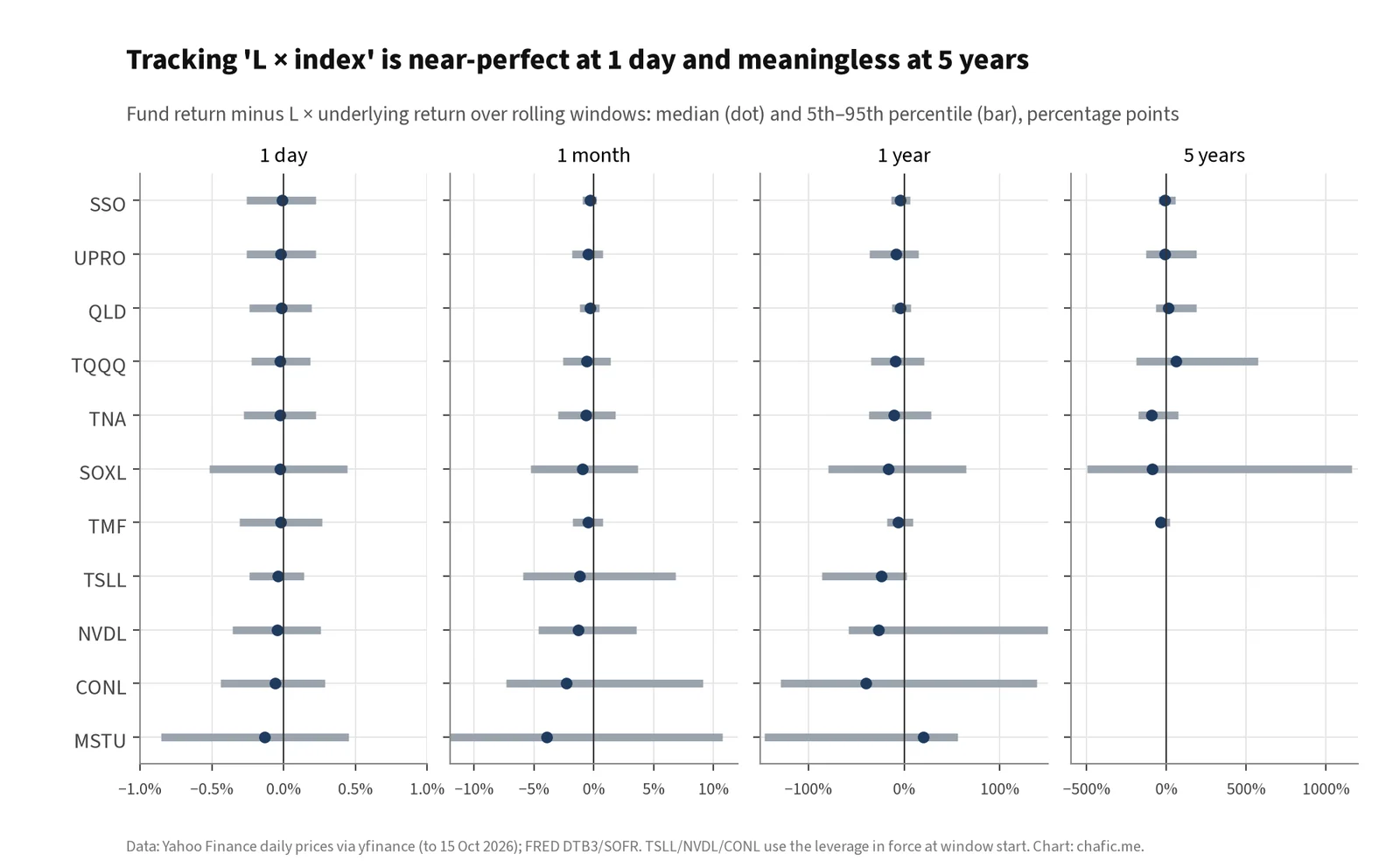
Figure 7. The same distributions for long funds. Note the change of scale across panels.
- One day: the funds do what they say. The median gap rounds to zero and 90% of days sit within about ±0.3pp for index funds. Daily correlation with the target exceeds 0.99 for every index fund.
- One month: a small, consistent shortfall of 0.3–0.9pp for long index funds, somewhat more compounding than cost. The range is still narrow.
- One year: long index funds trail L × index in 68–81% of windows, by a median of 4pp (SSO, QLD) to 16pp (SOXL). TSLL trailed in 95% of its 1-year windows.
- Five years: the median can be either sign (TQQQ +58pp, TNA −95pp), and the 5–95% range spans hundreds of points. Over this horizon “L × index” does not describe the product, because the outcome depends on the path.
Table 6 splits the median gap into compounding (frictionless daily reset minus L × index) and cost (fund minus frictionless reset). At one year compounding dominates; at five years the cost line alone is 9–77pp for long funds, and compounding goes positive for the trend-heavy Nasdaq-100 and S&P 500 funds while staying negative for small caps and semiconductors.
| Fund | 1y median gap | of which compounding | of which costs | 5y median gap | of which compounding | of which costs |
|---|---|---|---|---|---|---|
| SSO | −3.9 | −2.4 | −1.9 | −12.0 | +8.5 | −21.7 |
| UPRO | −8.3 | −5.7 | −3.0 | −9.7 | +26.5 | −41.2 |
| QLD | −4.2 | −2.1 | −2.3 | +12.4 | +39.9 | −31.4 |
| TQQQ | −9.0 | −6.3 | −3.6 | +58.5 | +117.6 | −66.1 |
| TNA | −10.9 | −8.4 | −3.0 | −95.4 | −73.7 | −22.2 |
| SOXL | −16.4 | −13.7 | −3.8 | −89.2 | −39.4 | −76.7 |
| TMF | −6.6 | −5.0 | −1.8 | −36.4 | −25.4 | −8.8 |
Table 6. Decomposition of the median rolling-window gap (pp). Medians are not additive, so the parts need not sum to the total.
When daily reset beats static leverage, and when it loses
The right comparison for a leveraged ETF is often not “L × index” but static leverage: borrow (L − 1) at the start, buy L of the index and do nothing. Static leverage drifts. It falls as the index rises and rises as it falls, and it can be wiped out. Daily reset holds exposure constant.
Under GBM the comparison has a clean shape. A daily-reset fund’s terminal value is S(T)L times a variance penalty: a convex function of the endpoint. Static leverage is linear in the endpoint. So the fund wins when the endpoint is far from the start in either direction and loses in a band around it. I call that band the “no-trend zone”. For 3× over one year it spans −11% to +27% at 15% volatility, −13% to +35% at 20%, and −18% to +55% at 30% (Figure 8). Most years fall inside it.
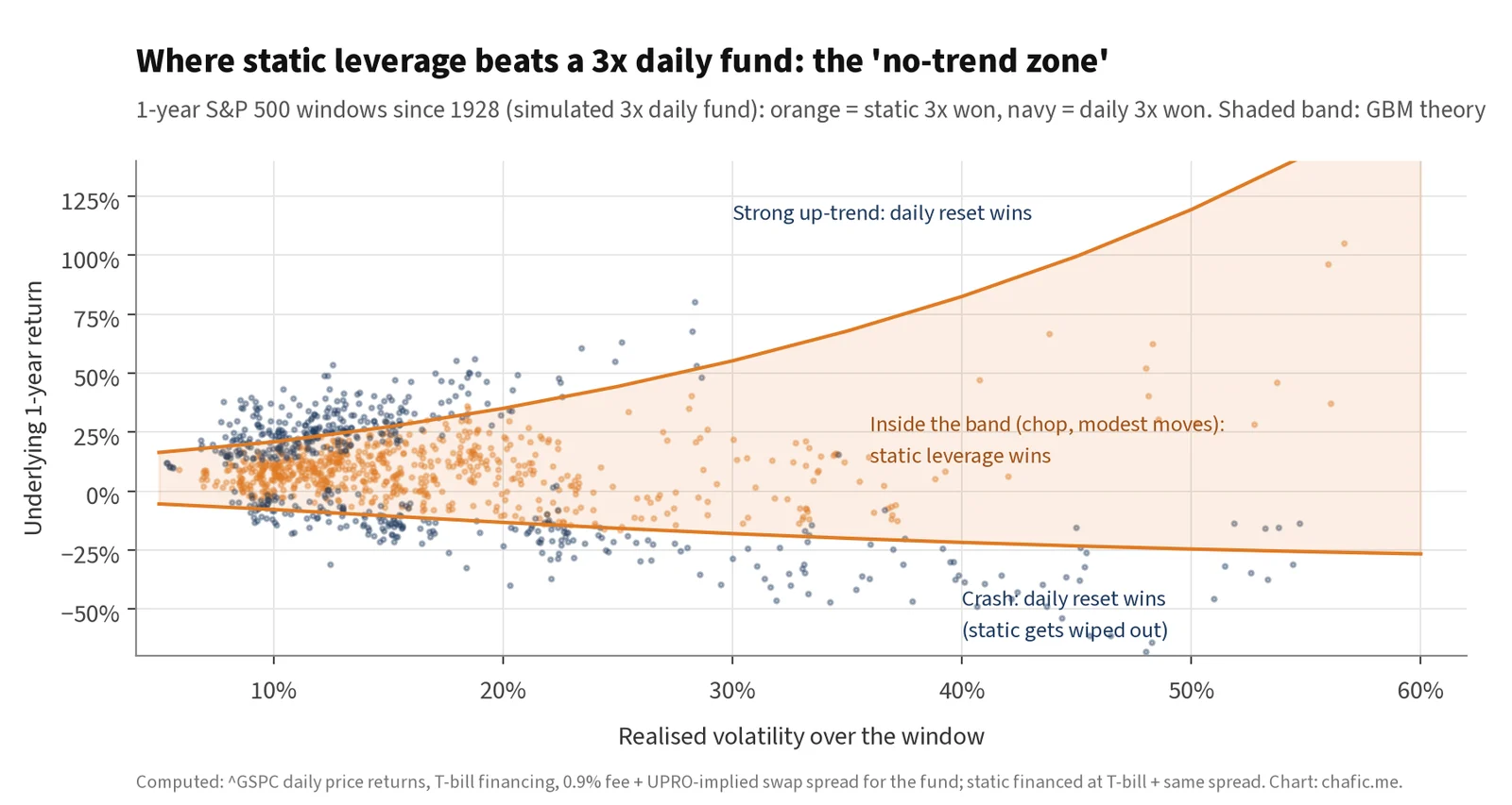
Figure 8. Daily 3× vs static 3× over every 1-year window of the S&P 500 since 1928 (simulated). The shaded band is the GBM no-trend zone.
Real funds show this pattern regime by regime (Table 7, Figure 9):
| Fund | Regime | Und. vol | Underlying | L × underlying | Static L (financed) | Fund | Winner |
|---|---|---|---|---|---|---|---|
| UPRO | 2010-19 low-vol bull | 15% | +255% | +766% | +754% | +1617% | daily |
| UPRO | 2015-16 chop | 17% | +1% | +3% | +2% | −9% | static |
| UPRO | Covid crash | 80% | −34% | −101% | −100% | −77% | daily |
| UPRO | 2020-21 rebound | 20% | +119% | +357% | +357% | +722% | daily |
| UPRO | 2022 bear | 24% | −19% | −56% | −60% | −58% | daily |
| UPRO | 2023-25 | 15% | +87% | +261% | +230% | +268% | daily |
| UPRO | 2026 YTD | 13% | +14% | +42% | +36% | +32% | static |
| TQQQ | 2010-19 low-vol bull | 17% | +429% | +1287% | +1276% | +4373% | daily |
| TQQQ | 2015-16 chop | 20% | −1% | −4% | −4% | −18% | static |
| TQQQ | Covid crash | 80% | −28% | −84% | −84% | −70% | daily |
| TQQQ | 2020-21 rebound | 23% | +136% | +408% | +408% | +834% | daily |
| TQQQ | 2022 bear | 32% | −33% | −99% | −100% | −80% | daily |
| TQQQ | 2023-25 | 20% | +138% | +413% | +383% | +548% | daily |
| TQQQ | 2026 YTD | 20% | +19% | +57% | +51% | +41% | static |
| SQQQ | 2010-19 low-vol bull | 17% | +429% | −1287% | −100% | −100% | tie (both ≈ −100%) |
| SQQQ | 2015-16 chop | 20% | −1% | +4% | +4% | −20% | static |
| SQQQ | Covid crash | 80% | −28% | +84% | +84% | +84% | daily |
| SQQQ | 2020-21 rebound | 23% | +136% | −408% | −100% | −96% | daily |
| SQQQ | 2022 bear | 32% | −33% | +99% | +107% | +89% | static |
| SQQQ | 2023-25 | 20% | +138% | −413% | −100% | −94% | daily |
| SQQQ | 2026 YTD | 20% | +19% | −57% | −45% | −45% | daily |
| TNA | 2010-19 low-vol bull | 19% | +203% | +608% | +597% | +546% | static |
| TNA | 2015-16 chop | 19% | −6% | −19% | −20% | −30% | static |
| TNA | Covid crash | 80% | −41% | −122% | −100% | −85% | daily |
| TNA | 2020-21 rebound | 28% | +129% | +386% | +386% | +644% | daily |
| TNA | 2022 bear | 28% | −21% | −64% | −68% | −64% | daily |
| TNA | 2023-25 | 21% | +48% | +145% | +114% | +51% | static |
| TNA | 2026 YTD | 18% | +13% | +38% | +32% | +22% | static |
| SOXL | 2010-19 low-vol bull | 24% | +504% | +1512% | +1501% | +2852% | daily |
| SOXL | 2015-16 chop | 25% | −2% | −6% | −6% | −25% | static |
| SOXL | Covid crash | 100% | −32% | −96% | −96% | −79% | daily |
| SOXL | 2020-21 rebound | 33% | +204% | +611% | +611% | +1363% | daily |
| SOXL | 2022 bear | 43% | −36% | −108% | −100% | −86% | daily |
| SOXL | 2023-25 | 35% | +171% | +513% | +482% | +359% | static |
| SOXL | 2026 YTD | 49% | +72% | +215% | +209% | +156% | static |
| TMF | 2010-19 low-vol bull | 14% | +99% | +298% | +286% | +245% | static |
| TMF | 2015-16 chop | 14% | +19% | +56% | +56% | +54% | static |
| TMF | Covid crash | 58% | +14% | +43% | +43% | +36% | static |
| TMF | 2020-21 rebound | 14% | −8% | −24% | −24% | −32% | static |
| TMF | 2022 bear | 20% | −29% | −88% | −92% | −70% | daily |
| TMF | 2023-25 | 15% | −3% | −9% | −39% | −49% | static |
| TMF | 2026 YTD | 10% | −5% | −15% | −21% | −23% | static |
Table 7. Leveraged ETFs vs L × underlying and vs static leverage financed at T-bills, by regime. Static leverage is floored at −100%. Underlying returns are total returns.
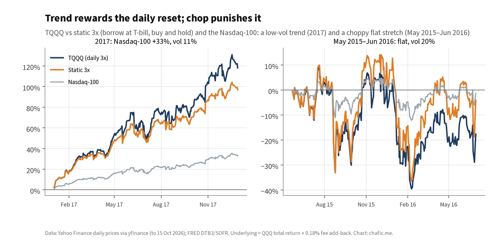
Figure 9. TQQQ in a low-volatility trend (2017) and in a flat, choppy stretch (May 2015–June 2016).
- Trending and low-volatility (2010–19, 2020–21 rebound, 2023–25): daily reset wins, often by multiples. TQQQ returned +4,373% over 2010–19 against +1,276% for static 3×, because positive compounding on a 17%-volatility trend outweighed the drag. UPRO returned +1,617% against +754%.
- Choppy and flat (2015–16): daily reset loses. Every long and inverse fund lost more than static leverage. TQQQ lost 18% and SQQQ lost 20% while the Nasdaq-100 moved −1%. Holding both legs lost money, which is the cleanest demonstration of decay.
- Crashes (Covid, 2022 for 3× tech, GFC): daily reset wins against static, but only because static leverage gets wiped out. TQQQ lost 80% in 2022; static 3× would have lost 100%. That is a win only on paper.
- Slow, volatile grinds (Russell 2000 2010–19 and 2023–25; semiconductors 2023–26): daily reset loses. TNA returned +546% over 2010–19 against +597% for static, and +51% against +114% over 2023–25. SOXL returned +359% against +482% over 2023–25 while the semiconductor index rose 171%.
- Inverse funds are the hardest case. In a rising market both inverse and static short lose most of the investment. The inverse fund’s daily reset is what keeps it above zero, but SQQQ still lost 94–100% in every multi-year bull window.
Over all 1-year windows since 1928, simulated daily 3× beat static 3× 46% of the time, and daily 2× beat static 2× 30% of the time. Over 5-year windows the 3× fund wins more often (63%), because over five years static 3× is more likely to have been wiped out or deleveraged by a trend (Table 8). The result also depends on the era. Lag-1 autocorrelation of daily S&P returns was −0.009 in 1928–69, +0.097 in 1970–99 and −0.100 in 2000–26. Daily reset is a momentum strategy at the daily frequency. When daily returns mean-revert, as they have since 2000, the reset buys after up days that are partly reversed, and 1-year windows ending after 2000 favoured daily 3× only 37% of the time.
| Window | L | Below L × index (simple) | Beats static L | …vol < 12% | 12–18% | 18–25% | > 25% |
|---|---|---|---|---|---|---|---|
| 1y | +2x | 88% | 30% | 26% | 32% | 26% | 39% |
| 1y | +3x | 81% | 46% | 51% | 44% | 36% | 48% |
| 1y | −1x | 22% | 29% | 29% | 32% | 20% | 28% |
| 1y | −3x | 28% | 39% | 45% | 44% | 25% | 30% |
| 5y | +2x | 86% | 37% | 30% | 42% | 20% | 63% |
| 5y | +3x | 81% | 63% | 59% | 68% | 54% | 72% |
| 5y | −1x | 21% | 36% | 40% | 45% | 24% | 17% |
| 5y | −3x | 22% | 55% | 55% | 58% | 54% | 43% |
Table 8. Share of rolling windows (S&P 500 1928–2026, simulated funds with 0.9% fee and UPRO-implied spread) in which the daily fund returned less than L × the index, and in which it beat static leverage, overall and by realised-volatility bucket.
Monte Carlo and historical rolling windows
The GBM results in Sections 2–3 isolate the mechanic. Two further checks relax the distributional assumption.
Block bootstrap of the S&P 500 (1988–2026). I resampled daily excess returns of the S&P 500 total-return index in blocks averaging 21 days, which preserves volatility clustering and fat tails. I added back today’s SOFR and ran 4,000 paths at each horizon (Table 9). A 3× fund’s median 1-year return was +23%, against a median +41% for 3× the index. The fund finished below 3× the index in 86% of paths, lost money in 33%, and beat static 3× in only 23%. Over five years the median 3× fund returned +128% against +247% for 3× the index. Inverse funds lost money in 75–98% of paths, because they carry both the drag and the equity premium against them.
| Horizon | L | Median fund | Median underlying | Median L × und. | P(fund < L × und.) | P(fund beats static L) | P(loss) | P(< −50%) |
|---|---|---|---|---|---|---|---|---|
| 1y | +2x | +19% | +14% | +27% | 92% | 18% | 28% | 1% |
| 1y | +3x | +23% | +14% | +41% | 86% | 23% | 33% | 4% |
| 1y | −1x | −9% | +14% | −14% | 3% | 28% | 75% | 0% |
| 1y | −3x | −34% | +14% | −41% | 26% | 38% | 85% | 25% |
| 5y | +2x | +112% | +82% | +165% | 82% | 26% | 15% | 3% |
| 5y | +3x | +128% | +82% | +247% | 78% | 30% | 22% | 10% |
| 5y | −1x | −36% | +82% | −82% | 0% | 56% | 91% | 21% |
| 5y | −3x | −88% | +82% | −247% | 12% | 69% | 98% | 93% |
Table 9. Stationary block bootstrap of S&P 500 TR daily excess returns (1988–2026), 4,000 paths, financing at SOFR 3.88%, 0.9% fee plus UPRO-implied spread. Static L financed at SOFR. Computed.
Long history (1928–2026). Using the S&P 500 price index from 1928, with T-bill financing (3-month bill; 2% assumed for 1928–33, before the FRED series starts), a simulated 3× daily fund lost −99.95% from September 1929 to June 1932, while the index lost −86%. On 19 October 1987 the index fell −20.5% and a 3× fund would have fallen −61.5% in one session. From 1934, price-only CAGRs were 7.4% for the index, 6.2% for 2× and 3.5% for 3×. All three lines exclude dividends. A real fund on a total-return index would also collect L × the dividend, so these CAGRs understate the levered lines. The comparisons between rebalancing rules in Section 9 are unaffected.
The sleeve under fat tails: bootstrap vs GBM
The August note’s main suggested upgrade was to replace GBM with each stock’s own returns. Table 10 does that. For eight of the sleeve’s underlyings with at least two years of history, I bootstrapped the last five years of daily returns (demeaned to zero drift, as in the original) and compared the 2× outcomes with GBM at the same volatility.
| Stock (last 5y) | Vol | Median 2x, bootstrap | Median 2x, GBM | Flat-year 2x, bootstrap | GBM | P(fund<0 given und>0), bootstrap | GBM | P(NAV wiped out), bootstrap |
|---|---|---|---|---|---|---|---|---|
| MSTR | 91% | −82% | −82% | −59% | −59% | 43% | 47% | 0.5% |
| COIN | 87% | −78% | −79% | −52% | −56% | 45% | 45% | 0.4% |
| MARA | 106% | −89% | −90% | −68% | −70% | 57% | 54% | 1.5% |
| IREN | 118% | −94% | −94% | −73% | −77% | 51% | 60% | 5.1% |
| CIFR | 122% | −96% | −95% | −77% | −79% | 64% | 62% | 8.2% |
| HOOD | 68% | −62% | −63% | −41% | −42% | 35% | 36% | 0.0% |
| SOFI | 66% | −62% | −61% | −38% | −39% | 34% | 35% | 0.0% |
| UPST | 102% | −90% | −89% | −62% | −68% | 51% | 52% | 18.7% |
Table 10. 2× daily fund on each stock’s own block-bootstrapped returns (last 5 years, demeaned, 4,000 paths) vs GBM at the same volatility (20,000 paths). Refreshed costs.
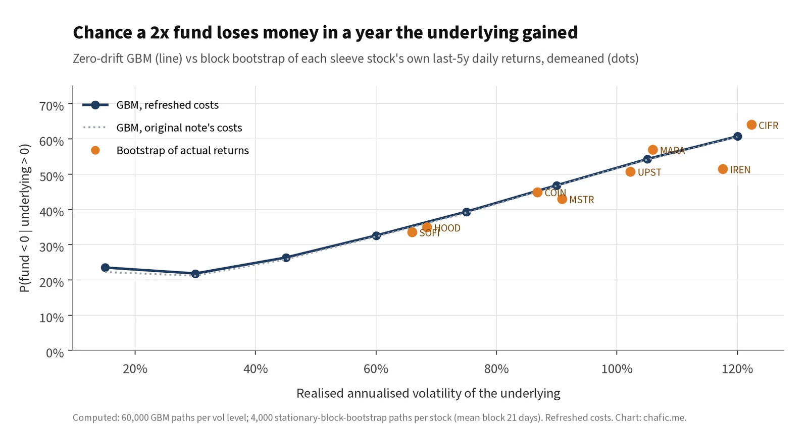
Figure 10. Probability that a 2× fund loses money in a year its stock gained: GBM (line) vs each stock’s own bootstrapped returns (dots).
The central results barely change. The median and the flat-year outcome are set by variance, and the bootstrap preserves variance. Negative-year probabilities move by a few points either way. What changes is the tail. The NAV is wiped out in 18.7% of UPST paths, 8.2% of CIFR, 5.1% of IREN and 1.5% of MARA, against essentially zero under GBM. The data contain single days of −56% (UPST), −47% (CIFR) and −36% (IREN). A 2× fund cannot survive the first of these.
Leverage factor against reset frequency
The August note’s most useful negative result was that lengthening the reset does not help. It holds up in simulation (Table 11, Figure 11). At 90% volatility, a flat year costs 58.5% with daily reset, 59.3% weekly and 60.0% monthly. At 120% the monthly variant is clearly worse (−84% against −78%), because the zero floor bites when 2× is applied to a large monthly fall. The leverage multiple is what changes the outcome: 1.5× loses 29% and 1.25× loses 14% at 90% volatility.
| Vol | Costs | 1.25x | 1.5x | 2x daily | 2x weekly | 2x monthly | 3x |
|---|---|---|---|---|---|---|---|
| 60% | note | −7.7% | −15.7% | −34.3% | −34.1% | −32.7% | −69.6% |
| 60% | refreshed | −8.1% | −16.1% | −34.6% | −34.5% | −33.0% | −69.8% |
| 90% | note | −13.9% | −28.8% | −58.3% | −59.1% | −59.8% | −92.6% |
| 90% | refreshed | −14.2% | −29.1% | −58.5% | −59.3% | −60.0% | −92.6% |
| 120% | note | −22.0% | −43.8% | −78.1% | −79.7% | −84.2% | −99.1% |
| 120% | refreshed | −22.3% | −44.0% | −78.2% | −79.8% | −84.4% | −99.1% |
Table 11. Median 12-month return on a flat round trip (±3%), 60,000 GBM paths per cell. “note” uses the August inputs; “refreshed” uses 0.45% fee, SOFR and a 1.0% spread.
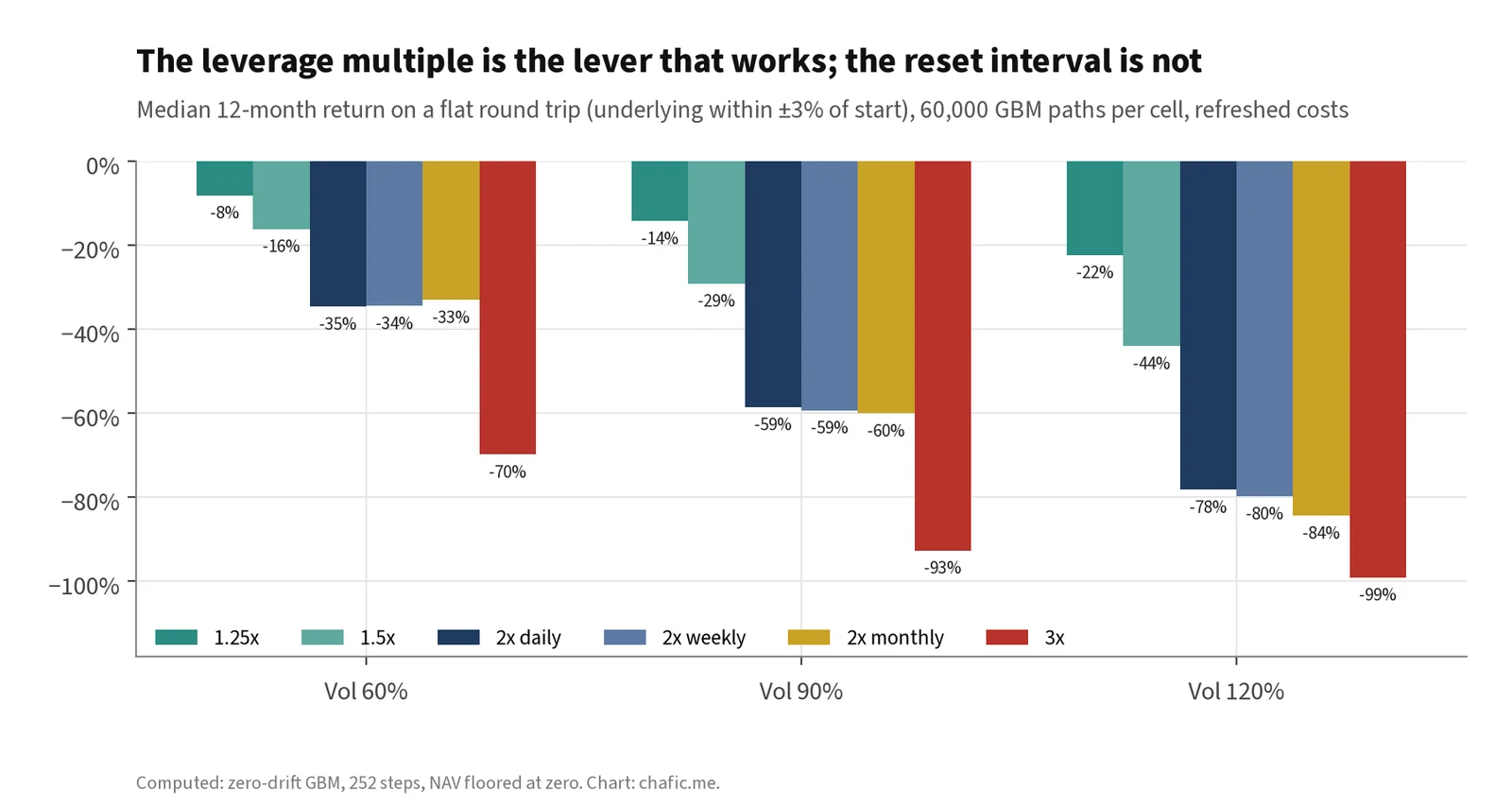
Figure 11. Leverage multiple vs reset interval, refreshed costs.
History agrees, and adds a warning (Table 12, Figure 12). Applying 3× to the S&P 500 from 1934 with financing at T-bills plus spread, daily, weekly and monthly rebalancing produced similar results (5.0–5.6% CAGR on price, worst drawdowns near −99%). Quarterly and annual rebalancing were wiped out, in November 2008 and October 1937 respectively. The longer a constant-leverage portfolio goes between rebalances, the larger the single move it must survive. Buy-and-hold static leverage did best over this particular sample, because a strong early rise (1934–37) let it deleverage before the 1937 crash. That result depends on the start date and should not be generalised. A volatility-targeted rule (scale exposure so trailing 21-day volatility is 20%, capped at 3×) cut the worst drawdown to −75% and raised the CAGR to 7.1%.
| 3x S&P 500 rule (1934–2026, price index) | CAGR | Max drawdown | Worst 12 months | Wiped out? |
|---|---|---|---|---|
| Daily | 5.0% | −98.7% | −92.7% | No |
| Weekly | 5.6% | −98.5% | −92.6% | No |
| Monthly | 5.2% | −99.0% | −95.1% | No |
| Quarterly | −100% | −100.0% | −100.0% | Nov 2008 |
| Annual | −100% | −100.0% | −100.0% | Oct 1937 |
| Buy-and-hold (static) | 8.7% | −96.3% | −85.0% | No |
| Vol-target 20%, cap 3x, daily | 7.1% | −74.7% | −58.1% | No |
| S&P 500 price index, 1x | 7.5% |
Table 12. 3× S&P 500 price index under different rebalancing rules, January 1934 – October 2026. Financing at T-bill + 0.53% spread, no fee. Computed.
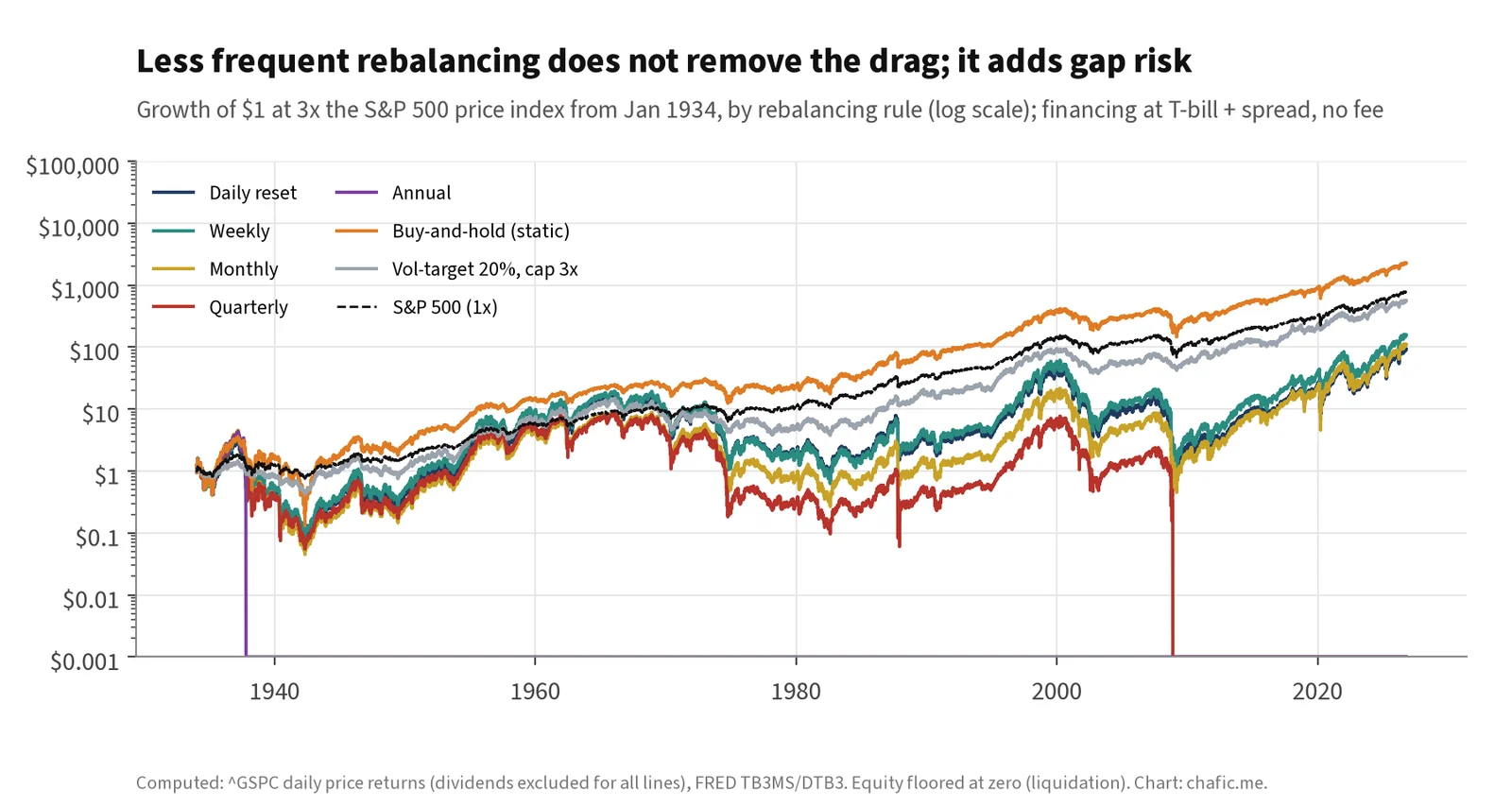
Figure 12. Growth of $1 under each rule (log scale).
Breakeven volatility
Setting the GBM log-growth rates against each other gives closed-form thresholds. With excess drift μ − r and annual cost c:
- The fund’s median beats the unlevered index if σ² < 2[(L − 1)(μ − r) − c] / (L² − 1).
- The fund’s median beats cash if σ² < 2[L(μ − r) − c] / L².
- Median growth peaks at L* = (μ − r)/σ², the Kelly leverage, before costs.
- Against the naive “L × index log growth”, the median never wins for L > 1. The gap is −(L − 1)r − c − ½(L² − L)σ², which is negative whenever rates are non-negative.
| L | Excess drift μ − r | Annual cost c | Median beats the unlevered index if σ < | Median beats cash if σ < |
|---|---|---|---|---|
| 1.5x | 4% | 1.7% | 7.0% | 19.6% |
| 1.5x | 6% | 1.7% | 14.5% | 25.5% |
| 1.5x | 8% | 1.7% | 19.2% | 30.3% |
| 2x | 4% | 2.0% | 11.7% | 17.4% |
| 2x | 6% | 2.0% | 16.4% | 22.4% |
| 2x | 8% | 2.0% | 20.1% | 26.5% |
| 3x | 4% | 2.5% | 11.7% | 14.5% |
| 3x | 6% | 2.5% | 15.4% | 18.6% |
| 3x | 8% | 2.5% | 18.4% | 21.9% |
Table 13. Breakeven volatility under GBM. μ − r is an assumption; c = 0.9% fee + |L| × 0.53% spread for index-type funds.
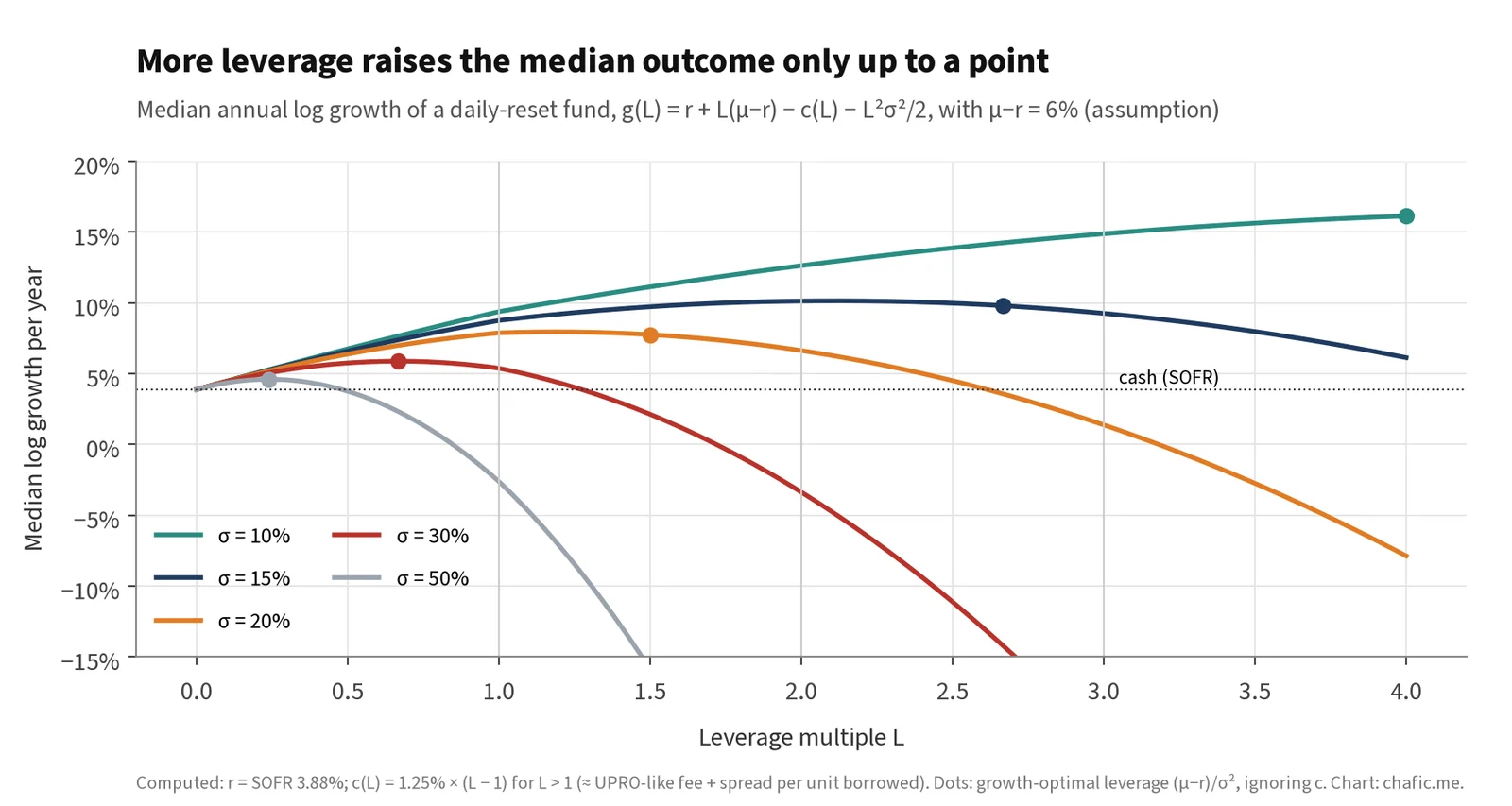
Figure 13. Median log growth against leverage for different volatility levels (μ − r = 6%, assumption).
At a 6% equity premium, a 3× fund’s median beats the index only when volatility is below about 15%, and beats cash only below about 19%. The S&P 500’s realised volatility over the funds’ lifetimes was 17–19% (Table 3). Broad 3× equity funds therefore sit almost exactly at their breakeven: they do very well in calm trends and badly in turbulent ones. At 16% volatility, the growth-optimal leverage is about 2.3×. On a single stock at 85% volatility with a generous 10% excess drift, it is 0.14×, and any leverage above roughly 0.3× lowers median growth below cash.
Gap risk
A 2× fund’s NAV is wiped out by a 50% fall in one session; a 3× fund by a 33.3% fall. Under the lognormal model those are extremely remote at index volatilities. Under the August note’s volatilities they are still remote in theory, once the sigma arithmetic is corrected:
| Vol | Daily s.d. | 50% fall in s.d. units: note (simple return) | Correct lognormal count, ln(0.5)/s.d. |
|---|---|---|---|
| 45% | 2.83% | 17.6 | 24.5 |
| 60% | 3.78% | 13.2 | 18.3 |
| 90% | 5.67% | 8.8 | 12.2 |
| 120% | 7.56% | 6.6 | 9.2 |
Table 14. Daily standard deviation and the size of a one-day 50% fall in standard deviations. The August note divided 0.5 by the daily s.d.; the lognormal count uses ln(0.5).
The data do not follow that model. Nine of the eleven sleeve underlyings have had at least one session of −20% or worse. MSTR, MARA and UPST have each had a session below −50% (Table 15). The 2× wrapper is one bad session from losing 40% or more, and history contains sessions that would end it. In practice, issuers’ prospectuses generally allow them to change or close a fund after extreme moves, and swap counterparties may reprice or withdraw lines under stress. Neither helps the holder on the day.
| Stock | Data from | Worst day | Date | Days ≤ −20% | Days ≤ −25% | Days ≤ −50% |
|---|---|---|---|---|---|---|
| MSTR | 1998-06 | −62% | 2000-03-20 | 15 | 8 | 1 |
| COIN | 2021-04 | −26% | 2022-05-11 | 2 | 1 | 0 |
| CRCL | 2025-06 | −20% | 2026-03-24 | 1 | 0 | 0 |
| MARA | 2012-05 | −71% | 2012-09-10 | 22 | 16 | 2 |
| BMNR | 2025-06 | −40% | 2025-07-09 | 3 | 2 | 0 |
| GLXY | 2025-05 | −17% | 2026-02-03 | 0 | 0 | 0 |
| IREN | 2021-11 | −36% | 2022-05-16 | 2 | 1 | 0 |
| CIFR | 2020-10 | −47% | 2022-05-10 | 4 | 1 | 0 |
| HOOD | 2021-07 | −28% | 2021-08-05 | 1 | 1 | 0 |
| SOFI | 2021-01 | −15% | 2026-04-29 | 0 | 0 | 0 |
| UPST | 2020-12 | −56% | 2022-05-10 | 4 | 4 | 1 |
Table 15. Largest single-day declines of the sleeve underlyings (full Yahoo Finance history; MARA and MSTR include pre-crypto history).
Volatility products
UVXY shows decay from a source other than compounding. It holds VIX futures, not the VIX, and in normal markets the futures curve slopes upward, so rolling from the front month to the second month loses money most months. VIXY, the unlevered version, turned $1 into $1.8 × 10⁻⁵ from October 2011 to October 2026 (CAGR −52%) while the VIX index itself fell from 40.8 to 16.5. UVXY adds leverage (2× until February 2018, 1.5× since) and therefore variance drag on top of an underlying with about 69% volatility. Its $1 became about $3 × 10⁻¹¹ (CAGR −80%). The inverse SVXY collected the roll yield for years and then lost 83% in one session in February 2018, after which it was cut to −0.5×.
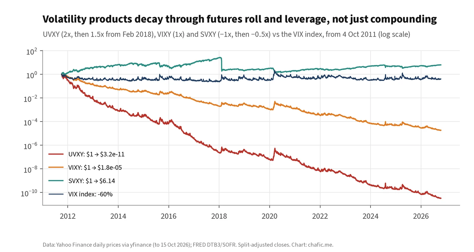
Figure 14. UVXY, VIXY and SVXY vs the VIX index, October 2011 – October 2026 (log scale).
Implications
13.1 Holding periods
- Days: the wrapper delivers what it promises. Tracking at one day is essentially exact for index funds. It is somewhat noisier for single stocks and VIX products because of close-versus-NAV timing.
- Weeks to a few months: the cost is roughly ½(L² − L)σ² × t plus financing. That is negligible on an index at 15% volatility (about 0.2% a month for 2×) and material on a single stock at 85% (about 6% a month for 2×). The investor is effectively short realised variance.
- A year or more: the outcome is a bet on the volatility regime and the shape of the trend, not on direction. It can beat L × index by a wide margin (UPRO, TQQQ) or fall far short (TNA, TMF). For single stocks above roughly 60% volatility, the expected median outcome is a large loss even when the investor is right about direction.
13.2 Alternatives
| Route to L× exposure | Financing cost (Oct 2026) | Path behaviour | Main risks |
|---|---|---|---|
| Daily-reset ETF | T-bill × (L − 1) + fee + swap spread: index ≈ 2–4%, single stock 7–34% beyond T-bills (Table 3) | Constant leverage, daily reset: short realised variance | Decay in chop; gap risk; fund closure |
| Margin account | IBKR Pro 5.38% (BM + 1.5%) up to $100k; Lite 6.38% [6]; full-service brokers higher | Static leverage unless rebalanced; Reg T limits initial leverage to 2× [7] | Margin calls at FINRA 25% maintenance [8]; forced selling at lows |
| Index futures (ES, MES) | Implied financing close to SOFR (basis varies; assumption) | Static per contract; leverage set by contracts per dollar of equity | Daily variation margin; roll; contract size (ES ≈ $387.2k, MES ≈ $38.7k notional at 7,744) |
| Deep ITM LEAPS calls | Embedded in time value: about 0.8–1.6% of spot for 70–80%-strike 1-year SPX calls (Table 16, assumed IVs) | Convex, no daily reset, no margin calls, maximum loss = premium | Delta falls in a sell-off; skew and dividends priced in; expiry |
| Constant-leverage portfolio (DIY) | Margin or futures rates | Same drag as an ETF if rebalanced daily; weekly/monthly similar; quarterly/annual risk wipe-out (Table 12) | Discipline; taxes; gap risk |
| Volatility-targeted leverage | Margin or futures rates | Leverage falls as volatility rises, cutting the variance term when it is largest | Model risk; whipsaw; lags sudden gaps |
| 1y SPX call strike | Assumed IV | Premium (% of spot) | Delta | Effective leverage | Time value (% of spot) |
|---|---|---|---|---|---|
| 60% of spot | 30% | 41.4% | 0.96 | 2.3× | 0.3% |
| 70% of spot | 27% | 32.2% | 0.93 | 2.9× | 0.8% |
| 80% of spot | 24% | 23.5% | 0.87 | 3.7× | 1.6% |
| 90% of spot | 21% | 15.3% | 0.76 | 4.9× | 3.1% |
| 100% of spot | 18% | 8.4% | 0.59 | 7.0× | 5.8% |
Table 16. Illustrative 1-year SPX call options under Black-Scholes, spot 7,744 (15 Oct 2026 close), r = SOFR 3.88%, q = 1.2%. Implied volatilities are assumptions shaped to resemble index skew. Effective leverage = delta × spot / premium. Time value = premium − (forward intrinsic), the embedded cost of financing plus the put protection the structure contains.
For a holder with a horizon beyond a few weeks, the cleanest substitutes are futures (cheap financing, no daily reset, no swap spread) and deep in-the-money calls (no margin calls, convex). Both require more account infrastructure than buying an ETF, which is the real service the ETF sells. A plain margin account at 2× is static leverage. It drifts, and it has the same wipe-out arithmetic.
13.3 What issuers could do
The August note ended with three recommendations addressed to an issuer. I keep their substance here as general product-design observations, since they apply to any issuer of single-stock leveraged funds:
- Publish a live drag figure. Show the trailing 30-day realised volatility of the underlying and the implied annual variance cost −½(L² − L)σ², updated daily, next to the fee. The fee alone understates the cost of holding. Disclose the swap spread too, since for single stocks it is the larger cost.
- Match the multiple to the volatility. On underlyings above roughly 75% volatility, 1.5× carries the drag of 2× on a 55%-volatility stock and keeps three-quarters of the exposure. That case rests on holders keeping positions for more than days, which only issuers’ own flow data can show.
- Monitor gap distance, not just exposure. Report the distance, in historical worst days rather than lognormal sigmas, to the single move that would end the fund.
Limitations
- Close-to-close prices, not NAV. Fund returns use market closes. For the small Corgi funds the premium or discount to NAV can be material over a few days and inflates measured tracking error. Their residual-cost estimates rest on 66–77 days and are not individually significant.
- Benchmark proxies. The S&P 500 uses ^SP500TR. The other benchmarks use their ETF’s adjusted close plus its fee, which approximates but does not equal the funds’ swap reference indices. VIXY is only a proxy for the S&P VIX Short-Term Futures Index.
- T-bill vs swap benchmark. Funds finance at swap benchmarks (SOFR, OBFR, Fed funds), not T-bills. Part of each “implied spread” is that basis.
- Long-history simulation uses the price index. Dividends are excluded throughout, and financing before 1934 is an assumed 2%. The 1929–32 and 1987 results are therefore illustrative of the mechanic, not of a product that existed.
- GBM, bootstrap and assumed parameters. Equity premia, implied volatilities for LEAPS and the 1.0% base-case spread are assumptions. Sensitivities are shown where they matter.
- Expense ratios are as reported by Yahoo Finance on 15 October 2026 and may differ slightly from current prospectuses.
- No view on any fund’s future performance. Nothing here is a recommendation to buy, sell or hold any security.
Appendix A. Full refreshed results
| Vol | Flat year, closed form | Flat year, simulated | Mean (analytic) | Median | P(fund<0 given und>0) | P(< −50%) | P(< −90%) | Break-even |
|---|---|---|---|---|---|---|---|---|
| 15% | −8.2% | −8.3% | −6.1% | −10.4% | 23.5% | 2.5% | 0.0% | 4.4% |
| 30% | −14.2% | −14.3% | −6.1% | −21.8% | 21.8% | 22.8% | 0.0% | 8.0% |
| 45% | −23.3% | −23.4% | −6.1% | −37.7% | 26.3% | 40.4% | 2.1% | 14.2% |
| 60% | −34.5% | −34.6% | −6.1% | −54.7% | 32.6% | 53.2% | 10.3% | 23.6% |
| 75% | −46.5% | −46.8% | −6.1% | −69.9% | 39.4% | 63.1% | 23.3% | 36.7% |
| 90% | −58.2% | −58.5% | −6.1% | −81.8% | 46.9% | 71.1% | 37.1% | 54.8% |
| 105% | −68.8% | −69.4% | −6.1% | −90.0% | 54.3% | 77.5% | 50.0% | 79.1% |
| 120% | −77.8% | −78.1% | −6.1% | −95.0% | 60.7% | 82.9% | 61.2% | 112.0% |
Table A1. 2× daily fund, zero-drift GBM, 60,000 paths, one year, refreshed costs (0.45% fee, SOFR 3.88% on borrowed notional, 1.0% spread on notional). Mean is the analytic population value exp(−cT) − 1; sample means are dominated by skew.
| Horizon | 15% | 30% | 45% | 60% | 75% | 90% | 105% | 120% |
|---|---|---|---|---|---|---|---|---|
| 1 month | −1% | −1% | −2% | −3% | −5% | −7% | −9% | −12% |
| 3 months | −2% | −4% | −6% | −10% | −14% | −20% | −25% | −31% |
| 6 months | −4% | −7% | −12% | −19% | −27% | −35% | −44% | −53% |
| 12 months | −8% | −14% | −23% | −35% | −47% | −58% | −69% | −78% |
| 24 months | −16% | −26% | −41% | −57% | −71% | −83% | −90% | −95% |
Table A2. 2× fund return on a flat round trip by horizon and volatility, refreshed costs (closed form; verified by simulation at 12 months).
Appendix B. Assumptions register
| Input | Status | Value and basis |
|---|---|---|
| Sleeve fees | Disclosed | 0.20% (MSTC, COIX, HOOC), 0.45% (others); issuer site and Yahoo Finance, 15 Oct 2026 |
| Financing benchmark | Observed | SOFR 3.88% (14 Oct 2026); 3-month T-bill 4.10% (FRED) |
| Swap spread, base case | Assumption | 1.0% on notional; real-fund evidence 0.5–1.2% (index) and 3–17% (single stock) |
| Index-fund simulations | Estimated | 0.9% fee + 0.53% spread per unit notional (UPRO residual) |
| Equity premium for breakevens | Assumption | 4%, 6%, 8% arithmetic excess return |
| Pre-1934 short rate | Assumption | 2.0% |
| LEAPS implied volatilities, dividend yield | Assumption | 18% at the money rising to 30% at 60% strike; q = 1.2% |
| Futures financing | Assumption | Close to SOFR; basis varies |
| Process | Model | GBM (Sections 2–3, 9, 10); stationary block bootstrap, mean block 21 days (Sections 7–8) |
Appendix C. Reproduction
Figures were produced with my own Python scripts from the public sources cited: prices from Yahoo Finance and rates from FRED. Random seeds are fixed. Each number in the text is recorded with its basis: computed, assumption or source.
References
- Corgi Invest, “Digital Asset & Crypto ETFs” and “Fintech ETFs” theme pages; fund page for COIX (fee, inception, swap-based exposure), retrieved 15 October 2026. https://corgiinvest.com/themes/digital-assets ; https://corgiinvest.com/themes/fintech ; https://corgiinvest.com/coix
- Yahoo Finance fund profiles (net expense ratio, inception) for all funds cited, retrieved via yfinance on 15 October 2026. https://finance.yahoo.com
- Direxion, “Direxion Announces Exposure and Risk Increase on Single Stock Daily Leveraged ETFs”, 2 February 2024; and Form 497K for TSLL (200% objective effective 2 April 2024). https://www.sec.gov/Archives/edgar/data/1424958/000119312524083681/d823444d497k.htm
- GraniteShares, “GraniteShares Amplifies Leverage in Single-Stock ETFs to 200%”, 22 January 2024 (NVDL, CONL), and Form 497. https://www.globenewswire.com/news-release/2024/01/22/2812991/0/en/graniteshares-amplifies-leverage-in-single-stock-etfs-to-200.html
- ProShares, change of UVXY’s objective to 1.5× and SVXY’s to −0.5× effective 28 February 2018; the change is also visible in the quarterly regression betas computed here.
- Interactive Brokers, “Margin Rates and Financing”, retrieved 15 October 2026. https://www.interactivebrokers.com/en/trading/margin-rates.php
- Board of Governors of the Federal Reserve System, Regulation T, 12 CFR §220.12 (supplement: margin requirements). https://www.ecfr.gov/current/title-12/chapter-II/subchapter-A/part-220
- FINRA Rule 4210, Margin Requirements. https://www.finra.org/rules-guidance/rulebooks/finra-rules/4210
- Federal Reserve Bank of St. Louis, FRED series DTB3, TB3MS and SOFR. https://fred.stlouisfed.org/series/SOFR
- CME Group, E-mini and Micro E-mini S&P 500 futures contract specifications. https://www.cmegroup.com/markets/equities/sp/e-mini-sandp500.contractSpecs.html
- Minder Cheng and Ananth Madhavan, “The Dynamics of Leveraged and Inverse Exchange-Traded Funds”, Journal of Investment Management 7(4), 2009.
- Marco Avellaneda and Stanley Zhang, “Path-Dependence of Leveraged ETF Returns”, SIAM Journal on Financial Mathematics 1, 2010.
- Alan Moreira and Tyler Muir, “Volatility-Managed Portfolios”, Journal of Finance 72(4), 2017.
- Chafic Charafeddine, “Two studies on Corgi’s leveraged and thematic shelf”, Part I, independent research, August 2026 (the study this note updates).